Whether you wish to use Niemeyer’s original geohash, Google’s S2, or Uber’s H3, FaunaDB’s flexible query language lets you drop in a variety of geospatial solutions.

Overview

It likely goes without saying, but I’ll state it anyway; if your product/organization isn’t utilizing geospatial data, you’re missing out. Even strictly internet-based companies will utilize geospatial data to aid in internationalization, customer insight, etc. As developers, when we think of geospatial capabilities in databases, we often share a similar set of critical questions.

Can my primary database handle geospatial data or do I need to add another database to my stack?

How does this database store geospatial data, if at all?

What sort of geospatial queries are possible?

Can this database scale in parallel with my primary database?

If you’re lucky and your primary database has geospatial capabilities, you still have to consider the possibility that those capabilities aren’t suited for your work; there’s a reason why Google and Uber have invented their own geospatial solutions. If you’re not so lucky, then you need to shop for a secondary database that’s “geo-enabled”. Of course, this comes with the typical scaling headaches: clustering, distributing, storing backups, etc. In addition, backend complexity is significantly increased by introducing ETL, another database driver at the API layer, capacity differences from the primary database, and more. All of this surface area for error leads to downstream consequences in your product and UX (e.g. delivery progress data is stale and the customer thinks the order is far away).

More often than not, when selecting geo-enabled databases, we opt for conventional databases with a shallow understanding of their geospatial capabilities. This happens when we prioritize maintainability over capability due to the database pains listed above, as a database that poorly addresses our objectives is better than a database that’s often down or irresponsive. Thus we arrive at what this piece is all about:

Using FaunaDB, we get a zero-maintenance database + the freedom to select from a variety of geospatial solutions :open_mouth: .

Zero-maintenance here means us developers don’t have to worry about sharding, replication, clustering, reserving read/write capacity, etc. We simply create a database and all the scaling and distribution is done behind the scenes. Now, I’m going to walk you through how my company, Cooksto, uses FaunaDB + Google’s S2 to build a location-based marketplace for homemade food.

Example Scenario

Imagine we have 25 meals that are being sold on the marketplace and a customer that only wants to browse food in walking distance (1000 meters or less). Now at this scale a simple distance calculation between the customer’s location and all of the meals isn’t much of a problem, however, we’re going to build with scale in mind for the sake of this walkthrough.

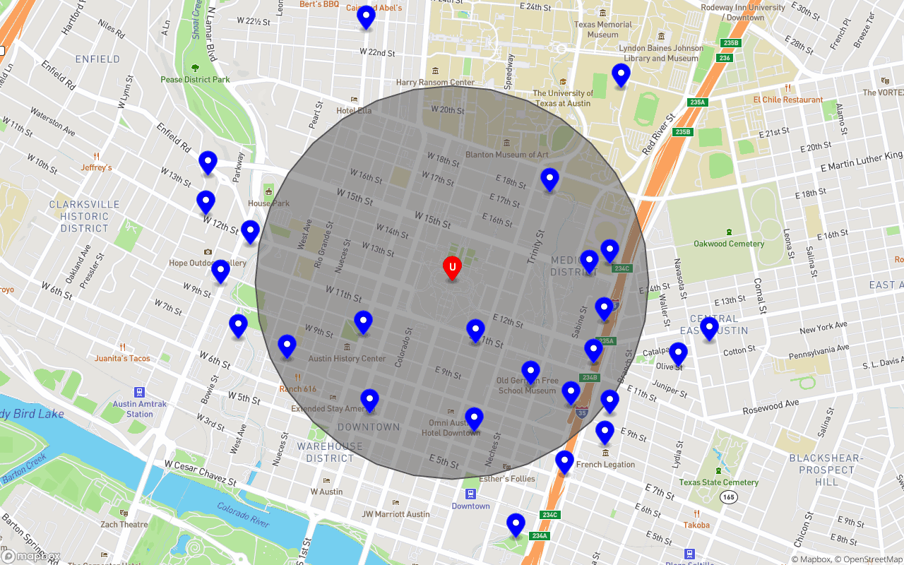
Our meals are represented with blue pins and white circles, while our user/customer is represented by the centered red pin and capital “U”. The gray circle illustrates the search radius (1000 meters). Our objective is to return only and all of the meals within the search radius.

Solution Part 1: Geohashes

When retrieving database entries based on a specific property, it’s often a good idea to utilize indexes (e.g. user by email). Indexing area/location however is significantly more complex than indexing an email or username field, as this sort of data often has a multi-dimensional representation (e.g. latitude & longitude, polygons, etc.). Encoding these multi-dimensional representations into singular strings or “hashes” is precisely the task geohashing was invented for.

Throughout this article I’ve used the term “geohash” sparingly for many geospatial indexing solutions (S2, H3, etc.) as it accurately describes the function of such solutions. However the exact meaning of “geohash” belongs to the very first solution of its kind, a library/system invented by Gustao Niemeyer in 2008. Since then though, Google has published a more accurate take (with respect to Earth’s sphere-like structure) on geohashes, called S2. I won’t go into too much detail about S2 here, so if you’re interested in reading more about S2 please refer to the official documentation. Below are a couple of images that summarize how S2 “works”.

Source: https://s2geometry.io/devguide/img/s2curve-large.gif. Roughly speaking, S2 projects a cube and its 6 sides onto our lovely planet, Earth :earth_americas: :heart: . Each of the six projected sides, numbered 0 - 5, is called a “face” and buckets a deep hierarchy of S2 “Cells”.

Source: https://s2geometry.io/devguide/img/s2hierarchy.gif. Every S2 Cell (the pseudo squares depicted above) encapsulates 4 children in a hierarchical manner (except the very last cells aka “leaf cells”, they have no children). This hierarchy of cells has a maximum depth of 30 levels, which at level 30 (the smallest representation of a space) is approximately a square centimeter.

There are many ways to represent an S2 Cell, but when used with FaunaDB, a “Hilbert Quadtree Key” (“quadkey” for short) is the optimal representation; this is due to how it represents the cell hierarchy and nesting with prefixes (more on this later). I first learned of this representation from an npm package called s2-geometry; in short, a quadkey is largely a base-4 number (i.e. most digits can only be 0 - 3) with only the first two characters not applicable to the base-4 property; the first character is reserved for the face (remember, a number inclusively between 0 and 5) and the second character is merely a forward slash (i.e. “ / “ ) to indicate separation between the face and cell numbers. Here’s an example maximum-length quadkey for an S2 Cell:

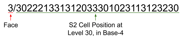
Due to base-4 representation and the fact that S2 Cells divide into 4 children at each level, each added digit represents 1 of 4 children and an increment in level. This allows us to prefix search on the quadkeys for broader/coarser results. Let’s briefly investigate this prefix property, between levels 5 and 9:

const { S2 } = require("s2-geometry");

const hawaii = {
  lat: 19.5968,
  lon: -155.5828,
};

console.log(
  "3/30222" === S2.latLngToKey(hawaii.lat, hawaii.lon, 5) &&
  "3/302221" === S2.latLngToKey(hawaii.lat, hawaii.lon, 6) &&
  "3/3022213" === S2.latLngToKey(hawaii.lat, hawaii.lon, 7) &&
  "3/30222133" === S2.latLngToKey(hawaii.lat, hawaii.lon, 8) &&
  "3/302221331" === S2.latLngToKey(hawaii.lat, hawaii.lon, 9)
); // true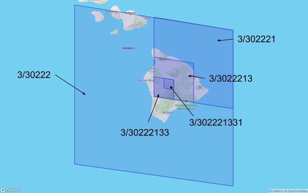

An image of S2 Cells covering Hawaii from levels 5 - 9. Hawaii can be contained within a quadkey of length 7, as can specific parts of the island if we enlarge the quadkeys to 7 + i, where i is some positive integer.

Due to base-4 representation and the fact that S2 Cells divide into 4 children at each level, each added digit represents 1 of 4 children and an increment in level.

Notice that lower levels are simply prefixes of the levels above them. This property applies to all levels. It’s precisely this prefix/nesting behavior that we’ll leverage when indexing our meals.

Solution Part 2: FaunaDB

Now that we have our indexing strategy (prefix searching our S2 Cell quadkeys/geohashes), let’s spin up our database resources. If you haven’t already, you’ll want to start by signing up at FaunaDB and creating a database (e.g. $ fauna create-database my_db; one of many ways to create a database, and yes, it’s really that easy).

After creating the database, we’ll need to create our collection. Recall that we’re providing a marketplace for homemade food, so we’ll name our collection “meals” (i.e. CreateCollection({ name: “meals”})). FaunaDB stores data in the form of nested document objects, each of which belong to a collection (the hierarchy looks something like Databases > Collections > Documents).

Data

It’s time to populate our collection, from here on I’ll be using the JavaScript driver for FaunaDB. Let’s create 25 meals within 1500 meters of our example customer:

const { query: q, Client } = require("faunadb");
const { randomCirclePoint } = require("random-location");
const { S2 } = require("s2-geometry");

const userCoordinates = { lat: 30.274665, lon: -97.74035 };
const searchRadius = 1000; // meters

// creates an array of 25 random points
const randomPoints = Array.from({ length: 25 }).map((num) =>
  randomCirclePoint(
    {
      latitude: userCoordinates.lat,
      longitude: userCoordinates.lon,
    },
    // * 1.5 to demonstrate excluding undesired results
    searchRadius * 1.5
  )
);

// creates an array of 25 meal objects in memory
const meals = randomPoints.map((point, i) => ({
  // usually something like "Marinara Pasta"
  name: `meal-${i}`,
  // ...
  // of course, in the real world, more attributes would go here
  // e.g. initNumServings, pricePerServing, etc.
  // ...
  pickupLocation: {
    // normally the meal's pickup address
    placeName: `placeName-${i}`,
    coordinates: { lat: point.latitude, lon: point.longitude },
    geohash: S2.latLngToKey(
      point.latitude,
      point.longitude,
      30 // max precision level, approximately a square cm
    ),
  },
}));

const client = new Client({
  secret: "<DATABASE_SECRET>",
});

// executes an FQL (Fauna Query Language) query
client
  .query(
    // creates a document in the "meals" collection
    // for each meal in the in-memory meals array
    q.Do(
      meals.map((data) =>
        // creates a document in the "meals" collection
        q.Create(q.Collection("meals"), {
          data,
        })
      )
    )
  )
  .then((data) => console.log(data))
  .catch((err) => console.log(err));

/*
Should console.log something like this:
[ { ref: Ref(Collection("meals"), "264247276731382290"),
    ts: 1588264691537000,
    data: { name: 'meal-0', pickupLocation: [Object] } },
  ...
  { ref: Ref(Collection("meals"), "264247276730322450"),
    ts: 1588264691537000,
    data: { name: 'meal-24', pickupLocation: [Object] } } ]
*/

Boom :boom: . We have a globally distributed database storing all of our meals. Let’s double-check our work and take a peek at the “meals” collection.

client
  .query(
    // maps over a page/array of 25 meal refs
    // e.g. Ref(Collection("meals"), "264069050122895891")
    q.Map(
      q.Paginate(q.Documents(q.Collection("meals"))),
      // given a ref, gets/reads the document from FaunaDB
      q.Lambda((ref) => q.Get(ref))
    )
  )
  .then((data) => console.log(data))
  .catch((err) => console.log(err));

/*
Should console.log something like this:
{ data: [
 { ref: Ref(Collection("meals"), "264069050122895891"),
   ts: 1588094720905000,
   data: [Object] },
 ...,
 { ref: Ref(Collection("meals"), "264145993260360211"),
   ts: 1588168099888000,
   data: [Object] }
] }
*/

Index

Obviously, querying the meals collection itself will return an undesired list of results. Recall that our customer only wants to browse meals that are within “walking distance” (1000 meters). In FaunaDB, whenever you want specific documents you utilize indexes. An index allows us to search and/or sort documents based on their fields. For example, we could create an index to match a given string with meal names, returning only those matched meals. In our case, we want an index that returns meals within a certain location, or more specifically, within a given S2 Cell.

For basic matching and sorting on fields as they are, you may simply create an index targeting those fields. However, if more complex matching/sorting is desired, then the logic that determines how or when to return specific results is stored within an index binding. In other words, given a source collection, an index binding provides a computed field(s) on each document for you to search and/or sort on. In our case, we want to compute a list of geohash prefixes to search on. For clarification, it’s indeed possible to search/sort on arrays (which is what we’re doing here), in addition to scalar values (e.g. a string). Let’s start with the “compute” logic for our index binding:

const minPrefixLength = 3;

// example max “prefix”: 4/030202112231011311302131301203
// two items to note:
// 1) maxPrefixLength represents the entire geohash
// 2) for simplicity sake, I consider the entire geohash...
// as a “prefix” in this code.
const maxPrefixLength = 32;

// a range of integers from 3 to 32
const allPossiblePrefixLengths = Array.from(
  { length: maxPrefixLength - minPrefixLength + 1 },
  (_, i) => minPrefixLength + i
);

// given a meal object or variable:
// returns an array of geohash prefixes
const computePrefixes = (meal) =>
  q.Let(
    {
      geohash: q.Select(["data", "pickupLocation", "geohash"], meal),
      prefixLengths: q.Take(
        q.Subtract(q.Length(q.Var("geohash")), minPrefixLength - 1),
        allPossiblePrefixLengths
      ),
    },
    q.Map(
      q.Var("prefixLengths"),
      q.Lambda((prefixLength) => q.SubString(q.Var("geohash"), 0, prefixLength))
    )
  );

// testing computePrefixes with a single meal
client
  .query(
    q.Let(
      {
        meal: q.Get(q.Documents(q.Collection("meals"))),
      },
      {
        geohash: q.Select(["data", "pickupLocation", "geohash"], q.Var("meal")),
        prefixes: computePrefixes(q.Var("meal")),
      }
    )
  )
  .then((data) => console.log(data))
  .catch((err) => console.log(err));

/*
Should console.log something like this:
{ geohash: '4/030202112231011311302131301203',
 prefixes:
  [ '4/0',
    '4/03',
    '4/030',
     ...
    '4/0302021122310113113021313012',
    '4/03020211223101131130213130120',
    '4/030202112231011311302131301203' ] }
*/

In essence, the binding takes a meal document and returns an array of prefixes, keep in mind that the last prefix in the array could be the entire geohash itself (which is technically not a prefix by definition). Now we just need to refer to our binding in our index creator, leaving us with:

// ...
// the initial variables from above...
// ...

const createPrefixIndex = q.CreateIndex({
  name: "meals_by_geohash",
  source: {
    collection: q.Collection("meals"),
    fields: {
      prefixes: q.Query(q.Lambda(computePrefixes)),
    },
  },
  // terms are what we search on
  terms: [{ binding: "prefixes" }],
  // values are what get returned
  // i.e. a meal's geohash, ref, latitude, and longitude
  values: [
    {
      field: ["data", "pickupLocation", "geohash"],
    },
    {
      field: ["ref"],
    },
    {
      field: ["data", "pickupLocation", "coordinates", "lat"],
    },
    {
      field: ["data", "pickupLocation", "coordinates", "lon"],
    },
  ],
});

client
  .query(createPrefixIndex)
  .then((data) => console.log(data))
  .catch((err) => console.log(err));

/*
Should console.log something like this:
{ ref: Index("meals_by_geohash"),
  ts: 1588263734990000,
  active: false,
  serialized: true,
  name: 'meals_by_geohash',
  source: ...,
  terms: ...,
  values: ...,
  partitions: 1 }
*/

Nice :slightly_smiling_face: . Let’s double check our work and test the index real quick.

// most of the meals we uploaded earlier...
// share the same geohash up to this prefix...
// so we should see multiple results
const coarseGeohash = "4/030202112231";

// again, multiple meals will likely share this geohash...
// however, less meals will likely be returned
const finerGeohash = coarseGeohash + "1";

const readIndex = {
  coarseGeohash: q.Count(q.Match(q.Index("meals_by_geohash"), coarseGeohash)),
  finerGeohash: q.Count(q.Match(q.Index("meals_by_geohash"), finerGeohash)),
};

client
  .query(readIndex)
  .then((data) => console.log(data))
  .catch((err) => console.log(err));

/*
Should console.log something like this:
{ coarseGeohash: 19, finerGeohash: 6 }
*/

Query

With our index created, it’s now possible to retrieve meals within an S2 Cell. If you recall, our customer wishes to browse meals within a specific search radius; when it comes to satisfying this search, we have a spectrum of granularity to choose from. In simpler terms, our search radius is a circle and we need to find one or more S2 Cells to cover/fill this circle. While using more S2 Cells (likely of varying sizes/levels) will more accurately mimic the shape of our search “circle”, it’ll also incur slightly higher costs. If extreme accuracy isn’t something desired, technically speaking, a single S2 Cell can cover our search radius, thus leading to a single read from our index. If moderate accuracy is something we’re okay with, then 4 ~ 8 S2 Cells should do the trick, resulting in (an insignificant) 4 ~ 8 index reads or less. This trend continues into the upper 10s of S2 Cells, where at this point, while the query will be extremely accurate, performance and cost should be considered.

The process of covering our search radius is a bit too detail intensive for this piece. Fortunately, FQL is a language that lends itself perfectly for query-generation which makes it easy for us to write higher-order FQL functions. With it, I’ve created an npm package called faunadb-geo, for us to use. One of the abstract FQL functions in the package, called GeoSearch, uses a series of Match, Range, and Difference operations to create the optimal FQL query under the hood. Typically, each read to the database would map to a single S2 Cell, but with FQL, I was able to save on performance and costs; optimizing a significant amount of reads to include more than one cell. I’ve included a handful of additional optimizations/adjustments you can select from, which affect the precision of your results, so I suggest exploring the docs/github repo for more info. Below is an example use of GeoSearch.

const { Client, query: q } = require("faunadb");
const { GeoSearch } = require("faunadb-geo")(q);

const userCoordinates = { lat: 30.274665, lon: -97.74035 };
const searchRadius = 1000; // meters

client.query(
  q.Paginate(
    GeoSearch("meals_by_geohash", userCoordinates, searchRadius, {
      maxReadOps: 8,
    })
  )
);

“Read ops” are how FaunaDB calculates costs per read, this is what’s referred to in the maxReadOps parameter. FaunaDB’s pricing is largely on-demand focused, however the opportunity to reserve read/write ops and more, in advance, is available. Fun fact: with the base pricing, a whole geoquery (from when it reads the indexes to when it reads each document) of 100 read ops easily undercuts the price of a “pro plan” Algolia search :clap: . It isn’t until the 300 read op range that the cost becomes similar; even then FaunaDB’s base pricing can be discounted as you scale.

Rather than log results, I’ve provided images of GeoSearch in multiple instances/coverings, demonstrating a spectrum of performances based on the maxReadOps parameter. Keep in mind that the actual number of read ops used will likely be less than what maxReadOps is set to.

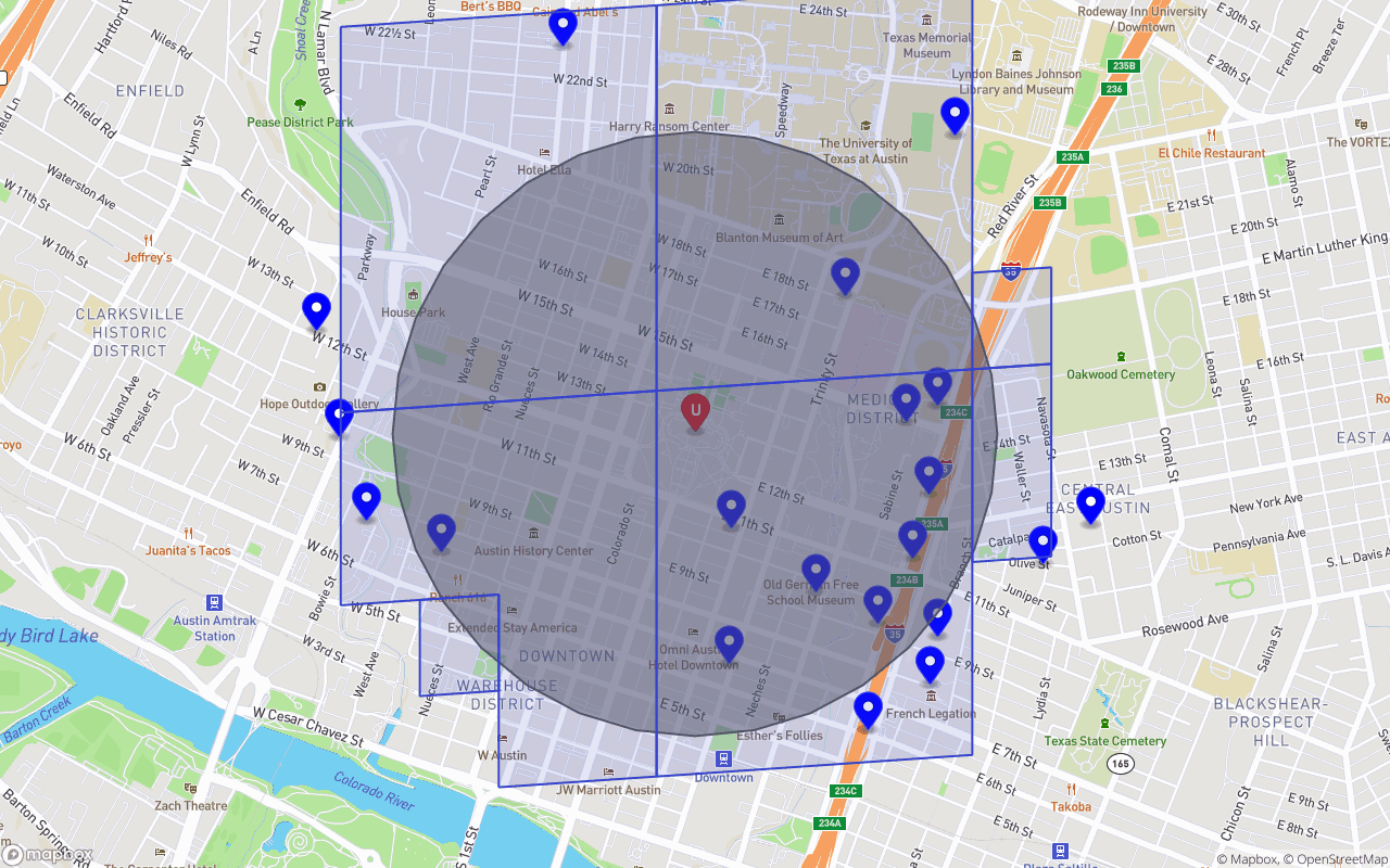
An image of S2 Cells and S2 Cell Ranges covering our customer’s search radius. A “Range” is just a series of neighboring/sibling cells we can combine under a single read. The blue polygons represent cells/cell-ranges we wish to read from our index, with each polygon resulting in a single read op. This particular covering had maxReadOps set to a mild 8.

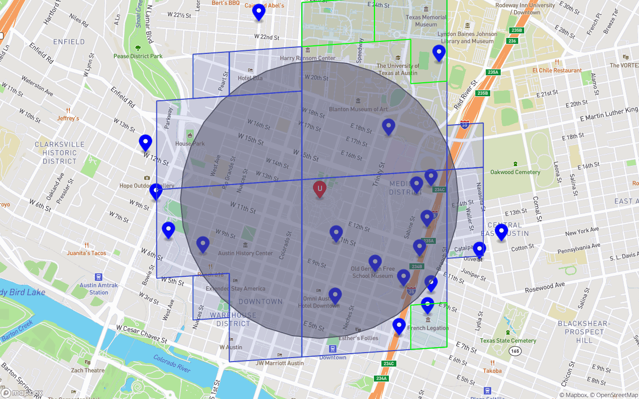
Green cells/cell-ranges represent cost efficient differences, used to reduce the total number of read ops. This covering had maxReadOps set to 16.

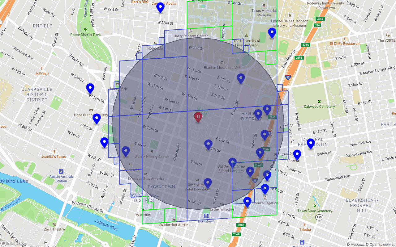
Another covering but with maxReadOps set to 32.

As you can see, our representation of the search radius can vary according to how many read ops we’d like to incur, along with how accurate we need our results to be. In the case of selling and advertising homemade food, the need for precision doesn’t necessarily outweigh the desire for cost effectiveness. In addition, using the CalculateDistance function from faunadb-geo, we can FQL Filter any results outside of our search radius (refer to the faunadb-geo docs for an example).

To conclude, with FaunaDB’s flexibility, both in implementation and performance, we’ve arrived at a solution which meets all of our needs. Our precision needs are satisfied with the ability to query across the planet or down to a few square centimeters. Any scale isn’t of concern to our globally-distributed database, where the concept of “instances” isn’t relevant to the developer. Additionally, our desire for cost effectiveness is easily accounted for with both a generous free-tier and very competitive on-demand pricing of FaunaDB (where in many cases our geoqueries are cheaper than alternatives like Algolia!). If you have any questions or comments, please feel free to reach out to me on the FaunaDB community slack. I hope you enjoyed this article and that FaunaDB excites you as much as it does for me, cheers! :beers: